Word2Vec from Scratch: How Neighbor-Prediction Turns Words into Geometry

Word2Vec has no notion of “meaning” — it only ever predicts which words sit near which, yet semantic structure falls out of that single objective. Here’s exactly why.

Background

Before dense embeddings, the default word representation was one-hot encoding: a vector of length V (the vocabulary size) that is all zeros except a single 1. Two problems follow immediately. The vectors are enormous and sparse — one dimension per word in the vocabulary — and, worse, every pair of distinct words is exactly equidistant. The dot product of any two one-hot vectors is zero, so “cat” is as unrelated to “dog” as it is to “the”. The representation carries no similarity information at all.

Word2Vec (Mikolov et al., 2013, “Efficient Estimation of Word Representations in Vector Space”) replaced this with dense vectors of 100–300 dimensions, learned so that geometric closeness encodes semantic relatedness. The bet it makes is the distributional hypothesis: words appearing in similar contexts tend to have similar meanings. The technical contribution was turning that linguistic observation into a cheap, self-supervised prediction task that scales to billions of words.

The Idea in Seven Steps

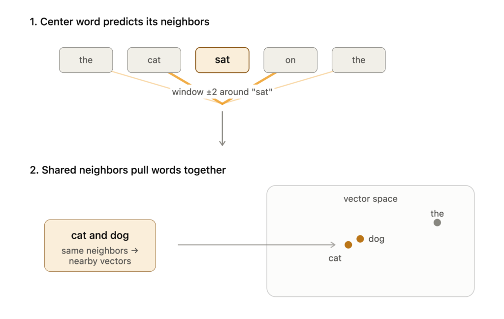
Before the matrices and gradients, here is the whole thing in plain language. Everything after this section is just these seven steps made precise.

Words become numbers. A computer can’t do math on the string “cat”, so we give every word a vector — a short list of numbers — and aim for similar words to end up with similar vectors.
Look at the neighbors. In the cat sat and the dog sat, “cat” and “dog” keep the same company. Words that share neighbors probably mean similar things. That single observation is the entire foundation.
Invent a guessing game. We can’t teach “meaning” directly, so we set a pretext task: given a word, guess its neighbors. We don’t care about the guesses — we care that getting good at them forces the model to notice that cat and dog behave alike.
Collect the practice material. Slide a small window over the text and write down every (word, neighbor) pair. the cat sat yields (cat, the) and (cat, sat). That list is the training data, extracted for free from raw text.
Nudge. For one pair, the model produces a guess, we measure how wrong it was, and we nudge the numbers a little: pull the real neighbor’s vector toward the center word, and push a few unrelated words away.
Repeat millions of times. One nudge does almost nothing. But cat gets pulled toward its neighbors and dog toward its neighbors — and since those neighbors are the same, cat and dog drift into the same region on their own. Meaning emerges from the accumulated pulls, not from any single step.
Use the vectors. Similar words now sit close together, so you can ask “what’s near cat?” and get dog, kitten, feline — by comparing directions with cosine similarity.

The rest of this post replaces the vague words in these steps — “nudge”, “a little”, “wrong” — with the exact matrices and gradients that implement them.

How It Works

The mechanism is a shallow network with no hidden nonlinearity — just two weight matrices. In the skip-gram variant, the task is step 3: given a center word, predict the words surrounding it within a fixed window. Nobody cares about the predictions; they are a pretext. The weights learned along the way are the actual product.

Each word gets two vectors, not one: a “center” vector in matrix W_in (shape V×D) and a “context” vector in W_out (shape D×V). The two-vector design isn’t arbitrary. A word acts in two different roles — as the word being looked at, and as a word appearing in someone else’s context — and the training objective only ever multiplies a center vector by a context vector, never a vector by itself. Collapse them into one vector and every word is structurally pushed to be its own best neighbor (since v · v = |v|² is always large and positive), which contradicts the data.

The forward pass for a training pair (c, ctx) is step 5’s “make a guess”: look up the center vector h = W_in (indexing a one-hot into a matrix is just a row selection, so no matrix multiply is needed), score it against every word with u = h @ W_out, and normalize with softmax into a probability distribution over the vocabulary. The loss is cross-entropy, -log(y[ctx]) — we want high probability on the true neighbor.

The elegant part is the gradient — the precise form of step 5’s “nudge”. Let e = y - onehot(ctx). For the true context word e[ctx] = y[ctx] - 1 is negative, which pulls that context vector toward h; for every other word e[j] = y[j] is positive, which pushes it away. Every step is a tug-of-war: attract the observed neighbor, repel everything else. Repeat across the corpus (step 6) and, because “cat” and “dog” get pulled toward the same set of context words, they converge to nearly the same region — without ever co-occurring. Semantic similarity emerges purely from shared neighbors.

Code

A complete, runnable skip-gram implementation with full softmax. The comments map each block back to the seven steps. This is deliberately the naive version — see the limitations section for why nobody ships this.

import numpy as np

corpus = [
    "the cat sat on the mat",
    "the dog sat on the log",
    "the cat chased the dog",
    "the dog chased the cat",
]

# --- Step 1 & 4: vocab (word <-> id) and skip-gram (center, context) pairs ---
tokens = [s.split() for s in corpus]
vocab = sorted({w for s in tokens for w in s})
w2i = {w: i for i, w in enumerate(vocab)}
V = len(vocab)

WINDOW = 2
pairs = []
for s in tokens:
    for i, center in enumerate(s):
        for j in range(max(0, i - WINDOW), min(len(s), i + WINDOW + 1)):
            if i != j:
                pairs.append((w2i[center], w2i[s[j]]))

# --- Two weight matrices: the two vectors per word from "How It Works" ---
D, LR, EPOCHS = 10, 0.05, 500
rng = np.random.default_rng(0)
W_in = rng.normal(0, 0.1, (V, D))   # row i = center embedding of word i
W_out = rng.normal(0, 0.1, (D, V))  # col j = context embedding of word j

def softmax(x):
    e = np.exp(x - x.max())         # subtract max for numerical stability
    return e / e.sum()

# --- Step 6: repeat the nudge over all pairs, many times ---
for epoch in range(EPOCHS):
    loss = 0.0
    rng.shuffle(pairs)
    for c, ctx in pairs:
        # Step 5a — make a guess
        h = W_in                 # (D,) look up center vector
        u = h @ W_out               # (V,) score against every word
        y = softmax(u)              # (V,) probabilities over vocab
        loss -= np.log(y[ctx] + 1e-10)

        # Step 5b — the nudge: pull the true neighbor, push the rest
        e = y.copy()
        e[ctx] -= 1.0               # (V,) dL/du
        grad_Win = W_out @ e        # (D,)  gradient for the center vector
        grad_Wout = np.outer(h, e)  # (D,V) gradient for all context vectors

        W_in -= LR * grad_Win
        W_out -= LR * grad_Wout
    if epoch % 100 == 0:
        print(f"epoch {epoch:4d}  loss {loss/len(pairs):.4f}")

# --- Step 7: use the embeddings — nearest neighbors by cosine similarity ---
E = W_in / np.linalg.norm(W_in, axis=1, keepdims=True)

def similar(word, k=3):
    v = E[w2i[word]]
    sims = E @ v                                    # cosine vs every word
    order = np.argsort(-sims)
    return [(vocab[i], round(float(sims[i]), 3))
            for i in order if vocab[i] != word][:k]

for w in ["cat", "sat", "chased"]:
    print(w, "->", similar(w))

On this toy corpus cat and dog come out close, because they occupy near-identical contexts — step 2’s shared-neighbor intuition made concrete. The final embeddings live in W_in; W_out is scaffolding and gets discarded.

Trade-offs & Limitations

The code above scores against all V words on every step: u = h @ W_out and the corresponding W_out update are both O(V·D). With V in the millions and billions of pairs, this is unusable. Real implementations replace the full softmax with negative sampling — reframing the problem as binary classification of “is this pair real?” against k (≈5–20) randomly drawn negatives, drawn from the unigram distribution raised to the 3/4 power. That makes the per-step cost independent of vocabulary size. Production Word2Vec also subsamples frequent words (discard with probability 1 - sqrt(t/f(w)), t≈1e-5) and randomizes the window size per center word. The deeper limitation is architectural: one vector per word means “bank” (river) and “bank” (money) are collapsed into a single averaged point. Word2Vec has no notion of context at inference — the vector is a static lookup — which is precisely the constraint that contextual models were built to remove.

My Take

Word2Vec is worth implementing by hand exactly once, because the skeleton — training pairs, a dot-product score, a softmax, and an attract/repel gradient — is the same structure underneath contrastive learning, modern embedding models, and the input embedding table of every transformer LLM. You will almost never train it from scratch in practice; grab pretrained fastText vectors (which handle morphology and out-of-vocabulary words via subword pieces, and matter more than plain Word2Vec for compounding languages like German). But understanding why neighbor-prediction produces geometry is what makes the entire embedding-based half of modern NLP legible rather than magical. Learn the intuition and the data flow; let the library compute the gradients.

Tags: Machine Learning, NLP, Embeddings, Python

Get in Contact